


Asprova Beginner's Lesson 5 -- Finite Capacity --
30 minutes
Learn by Movie
Download the project file of this lesson.
If you take a look to the documentation, please read the following.
What you will learn in this lesson
In this lesson, you will learn how to schedule operations with finite capacity by taking the number of production equipment and number of operators into account and automatically schedule the production sequence. Then, feasible work instructions will be exported from Asprova.
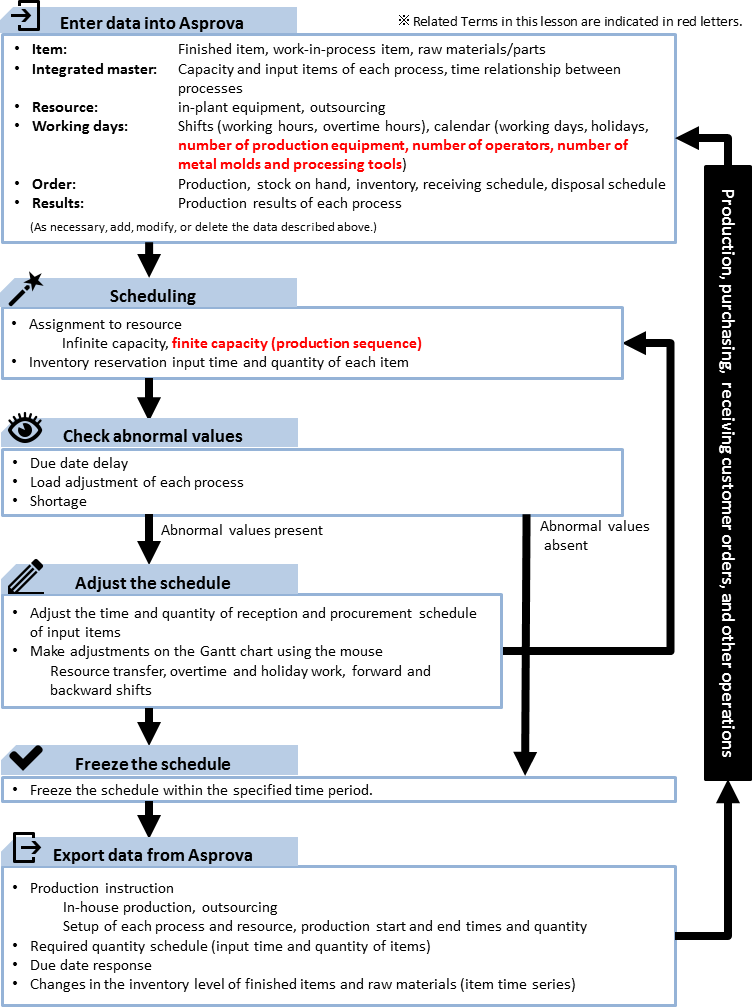
The following figure illustrates the assumed workflow. What is different about this workflow from the previous workflows is that finite capacity scheduling will be executed automatically.
The contents of this lesson apply to MS Light and higher modules, and the operations described here are for the MS Light module. For information on how to switch the module, see "How to start Asprova"
Download the project file of this lesson.
If you have questions, please access "Q&A Center" from navigation menu of this web site.
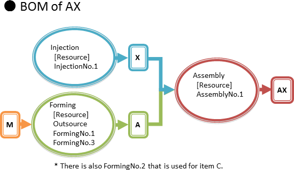
BOM (bill of materials) used in this lesson
This lesson assumes that the aforementioned workflow is performed on a daily basis.
The forming process uses three pieces of equipment. Since there is not enough in-plant equipment to cover all the production, some of it is outsourced. About three jobs can be outsourced in parallel. It is possible to outsource more jobs, but this could lead to problems if the production quantity is increased. Therefore, we keep the number within three when we schedule.
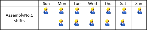
The assembly process is run by two operators from Monday to Friday and one operator on Saturday and Sunday.
Procedure
1. Entering Data into Asprova
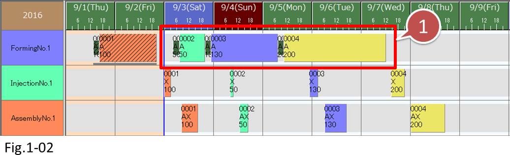
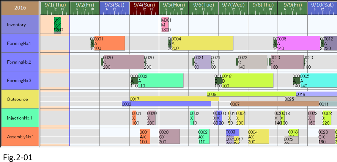
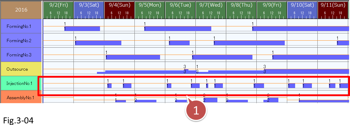
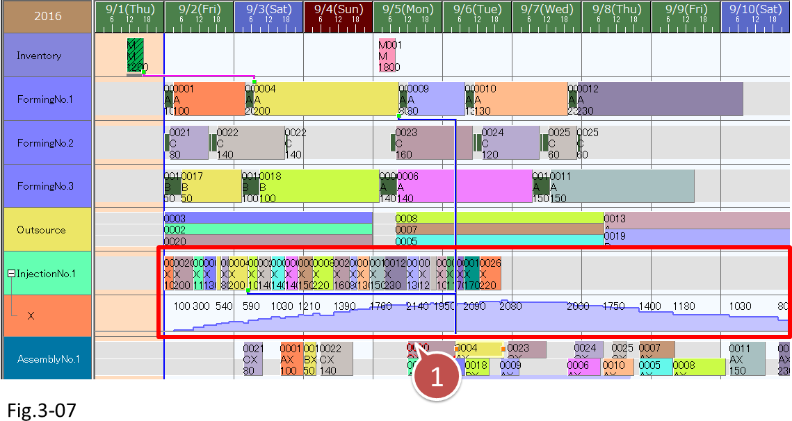
Set the number of equipment and number of operators as [Resource quantity] for each resource. Up to lesson 4, we used infinite capacity scheduling, which does not take resource quantity constraints into account. Consequently, schedules sometimes had stacked operations as shown in the figure below.
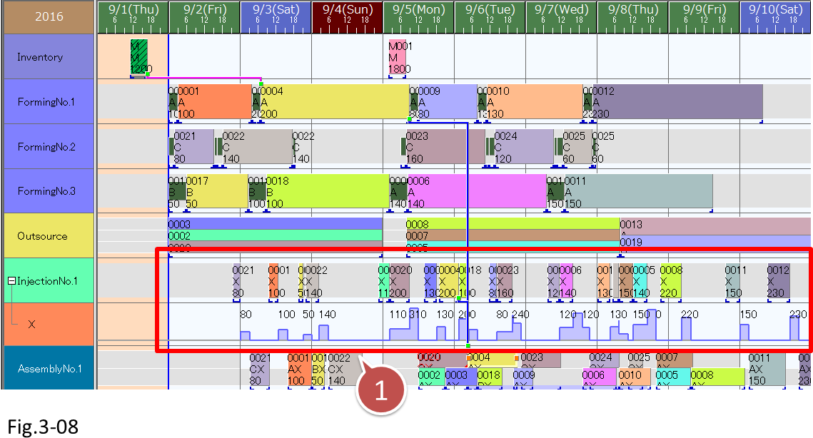
With finite capacity scheduling, operations can be assigned so that specified resource quantities are not exceeded, as shown in the bottom figure.
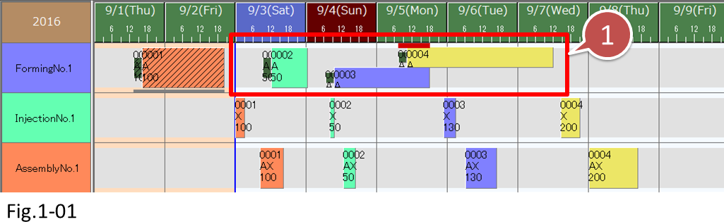
- With infinite capacity scheduling, the number of equipment and other resource quantity constraints are not taken into account, so operations may be stacked.
- With finite capacity scheduling, operations are assigned so that resource quantities specified in the calendar (the number of operators and equipment) are not exceeded.
1-1. Entering Data in the Calendar
We use the Calendar table to set shifts and resource quantities for each resource on a daily basis. We can specify working hours flexibly by setting ranges of days or specific weekdays and by setting the number of equipment or operators for resource quantities.
■ Steps
(1) Display the calendar table.
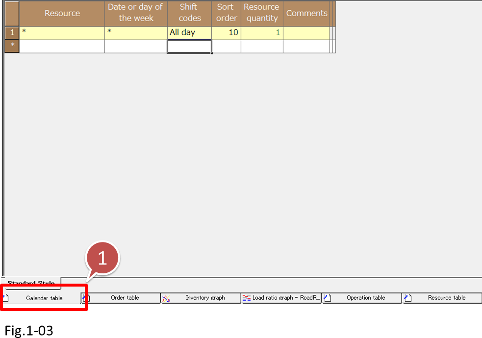
- Click Calendar table.
(2) For each calendar item, set the data as shown in the right figure.
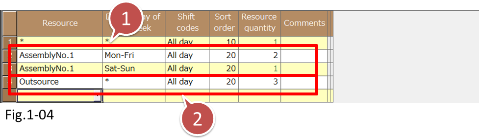
- For Assembly No.1, assign two operators for the Monday to Friday shift and one operator for the Saturday and Sunday shift.
- Set the resource quantity of [Outsource] to 3.
We set the resource quantity for AssemblyNo.1 in the calendar to 2 because there are two operators. We set the resource quantity of Outsource to 3 since up to three jobs can be outsourced in parallel.
Examples for setting resource quantities
To accommodate specific features of production equipment or to manage production equipment or operators in groups, you can set the resource quantity in the following manner.
- ● If there is a piece of equipment that can handle multiple instructions simultaneously
- Machining center or other pieces of equipment, which have multiple production arms or multiple lanes, that can handle two operations simultaneously
- -> Set the resource quantity to 2.
- ● If specific resources are handled collectively as a group
- Three production machines managed as one resource
- -> Set the resource quantity to 3.
- Five operators managed as one production department resource
- -> Set the resource quantity to 5.
(3) Let's check the Resource Gantt chart after we finish entering the data. Each resource is displayed in divided rows according to the resource quantity specified in the calendar.
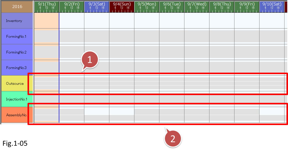
- Since the resource quantity of [Outsource] is 3, the resource is divided into three rows.
- For Assembly No.1, two operators are assigned for the Monday to Friday shift and one operator is assigned for the Saturday and Sunday shift.
2. Scheduling
2-1 Finite Capacity Assignment
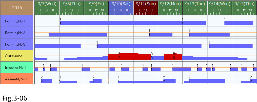
If we execute a reschedule with the scheduling parameter set to [Backward scheduling], a schedule is created so that resource quantity constraints are met. Since the resource quantities of AssemblyNo.1 and Outsource are 2 and 3, respectively, some operations are stacked.
- Assigned on the basis of the calendar resource quantities and resource quantity constraints so that resource quantities are not exceeded.
Creating an entire schedule with finite or infinite capacity
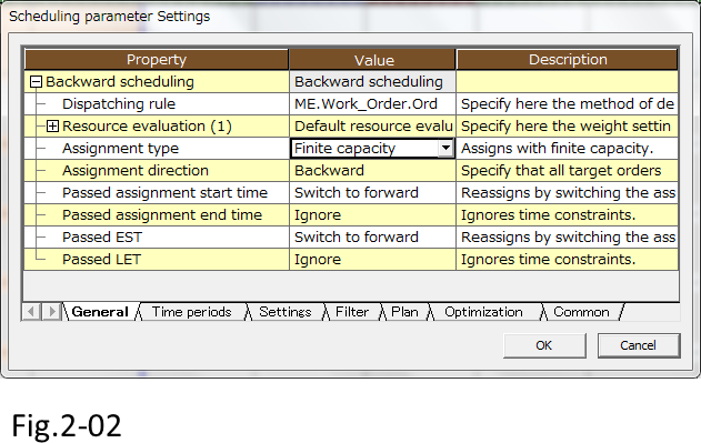
You can select whether to use finite capacity scheduling
with the [Assignment type] scheduling parameter.
- You can display the scheduling parameters by clicking [Scheduling Parameter Settings] on the [Schedule] menu.
- For MS Light, the Scheduling parameter option is required.
If you select [Infinite capacity], the schedule is created with infinity capacity.
Select finite or infinite capacity depending on your purpose.
-> For details, see lesson 10, "Scheduling Parameter.
3. Checking Abnormal Values
Let's check the schedule results for due date delays and unnecessary wait times between processes.
To check the information about the entire schedule, display the schedule evaluation result table. Choose [Table View]-[Evaluation Result]-[Schedule].
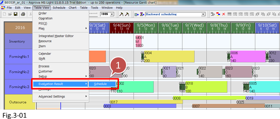
- Choose [Table View]-[Evaluation Result]-[Schedule]
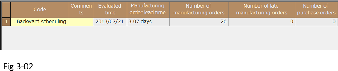
The schedule evaluation result table displays number of manufacturing orders, number of late manufacturing orders, manufacturing order lead time average, and other information. Since a history of past schedule results will be saved, if you see great changes, check for possible reasons.
If there are late manufacturing orders, make adjustments with the mouse on the Resource Gantt chart, as you did in lesson 4 and earlier lessons.
3-1 Checking the Load
Use the load graph to check the load conditions of processes and resources. You will be able to accurately grasp the load ratio of each resource, the number of outsourced jobs, and so on in order to increase operators, adjust the working time of equipment, and execute other measures in advance.
There are two types of Load graphs: Load ratio graph and Load amount graph.
The Load ratio graph displays the ratio of the time and resource quantity that are assigned to operations to the working time entered for the shifts in the calendar. The Load amount graph displays the resource quantities entered in the calendar and the resource quantity used in each operation.
■ Steps to check the load
(1) Display the load graph. Click the [Load Ratio] tab to display the load ratio graph. Checking the load ratio, we can see that the Forming resource load is higher than the load on other process resources.
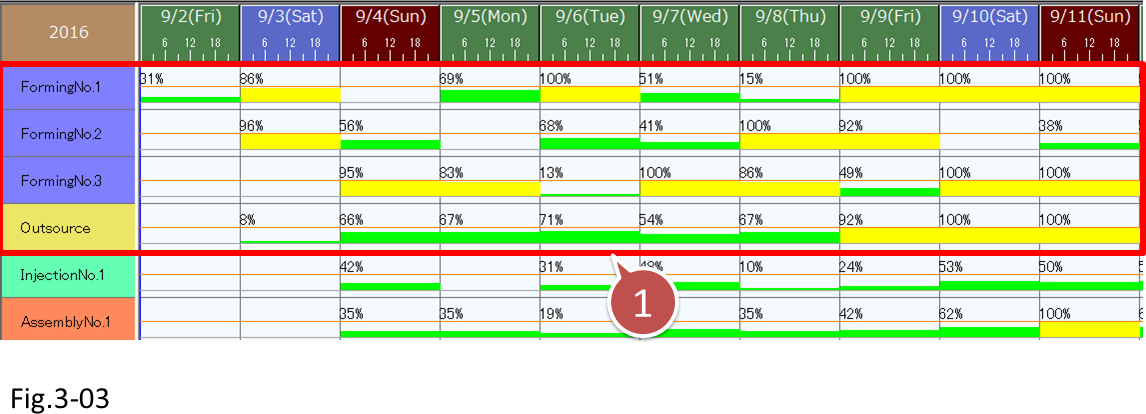
- Check the load ratio of each resource on the Load ratio graph.
(2) Next, click the [Load Amount] tab to display the Load amount graph. Recall that we set the maximum number of outsourced jobs to 3. On the graph, we can see when and how many jobs will be outsourced. For AssemblyNo.1, we can see how many operators are actually required in comparison to the two-operator or one-operator shifts that we specified for specific weekdays on the calendar.
- Since the Load amount graph displays how much of the resource quantities specified on the calendar is used, we can view the number of outsourced jobs and other related information.
Making only specific resources infinite capacity when scheduling
There are occasions when we want to assign a portion of the resources with infinite capacity when the entire schedule is created with finite capacity.
An example of such resources would be outsource resources that have no resource quantity constraints.
In such a case, set the [Resource quantity constraints] parameter in the resource table to [Not constrained].
Set this parameter appropriately depending on the characteristics of each resource.
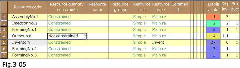
- Even in finite capacity scheduling, you can assign a portion of the resources with infinite capacity.
3-2 Checking the Wait Time between Processes
The wait time between processes affect lead time. Lead time refers to the time period from when raw materials and parts are loaded to when the production of finished items is completed.
If the amount of work-in-process inventory is large or when wait time is long, the increase in work-in-process inventory quantity becomes clearly noticeable on the Inventory graph, as shown in the right figure. (This schedule is using [Forward scheduling].) A large work-in-process inventory indicates a high possibility that the corresponding process or the previous or following process is causing a bottle neck.
- If the amount of work-in-process inventory is large or when wait time is long, the increase in work-in-process inventory quantity becomes clearly noticeable on the Inventory graph.
This is easy to verify by displaying the details of the Inventory graph on the Resource Gantt chart. Then, you can shift the relevant operation forward or backward as necessary. If you want to verify all items, use the Inventory graph.
- Shift the relevant operation forward or backward as necessary.
When you finish checking the schedule results, check and adjust the operations if necessary, and export the work instructions for each process (as you did in lesson 4 and earlier lessons).
Related Materials
For more details, see the following materials.